Day 20: Board Meeting & Free Fall

Physical Science: Newton’s Laws Board Meeting

Students finished collecting data, then we had a short board meeting to agree on the qualitative relationships in Newton’s 2nd Law.

Physics: Free Fall

Students white boarded answers to a few qualitative questions about last week’s Direct Measurement Video. I emphasized having them provide evidence to support their answers, which lead to some good conversations, both in groups and in the whole class, about what makes “good” evidence. Different groups looked at different combinations of falling objects, which lead to some good disagreement about whether all objects fell at the same rate. My favorite moment was when I asked whether using the same acceleration for all objects is useful and a student quickly responded with “It depends” which lead to some good talk about uncertainty.

Day 19: Newton’s 2nd Law & Constant Acceleration Practical

Physical Science: Newton’s 2nd Law

Students began collecting data for Newton’s 2nd Law using the classic modified Atwood’s machine. This is the first time students have done an open-ended lab with quantitative data, and I enjoyed watching groups tweak their experiment to get good data.

IMG_1204

This group added mass to slow their cart down, then added the golf ball to prevent it from sliding around in case that impacted the motion.

Physics: Constant Acceleration Practical

Students finished the practical started on Wednesday. After we collected data as a class to determine the speed of a tumble buggy and the acceleration of a marble on a ramp, each group got a starting position for either the marble or the buggy. Groups then had to figure out where to start the other so that, when released at the same time, the marble would land in a cup on top of the buggy.

Day 18: Intertia & Free Fall

Physical Science: Inertia

After some brief notes on inertia, students did a lab where they played with some examples and practiced using inertia to explain their observations. At the end of the lab, students had a mini-design challenge to come up with a way to keep the passenger safe in a collision. Even though we don’t go into torque in the course, it did get students thinking about where the force is applied. I intentionally left the language in the question vague, and I was pleased with the conversations students had about what it meant to keep the passenger safe.

IMG_1202

This group debated about the efficacy of their “seat belt” since the passenger’s “feet” still swung forward in the crash

Physics: Introducing Free Fall

We went to the computer lab for students to use a Direct Measurement Video to begin exploring free fall. This one allows students to watch side by side high speed videos of a variety of objects in free fall. I asked students to find a value for the acceleration of a falling object and to identify any variables that affects that acceleration. While many students were quick to dismiss small differences in the time, one group had a great discussion. They saw that the bowling ball fell noticeably faster than a ping pong ball, so they not surprisingly decided that weight must matter. One person wasn’t satisfied; he played the video of a large steel ball side by side with a small steel ball to show they fell at the same rate in spite of different masses and radii. With some nudging, they were able to agree that density must be the key factor.

IMG_1203

Day 17: Weight & Acceleration Practical

Physical Science: Weight

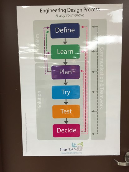
Today began with some talk about the engineering design process developed by EngrTEAMS. In particular, we placed ourselves in the “Learn” phase since students agreed they need some new science to understand crashes. I introduced forces as a tool for understanding crashes, and we dove in to a lab where students used spring scales to measure the weight of several hanging masses, then graphed the results. Tomorrow, we’ll get to the idea that the slope is the strength of gravity.

Since the lab is fairly straightforward, I had the chance to do one-on-one conferences with a few students who currently have low grades to make an action plan. I’m taking an “SBG-ish” approach in the course, which means I enter unit tests in the gradebook, rather than standards, but the tests are nearly all of the grade and I allow retakes to replace the initial score. I really liked that this freed me to talk with students about missing skills and understandings, rather than a long list of missing assignments. The students also seemed much more positive about these conferences than in the past.

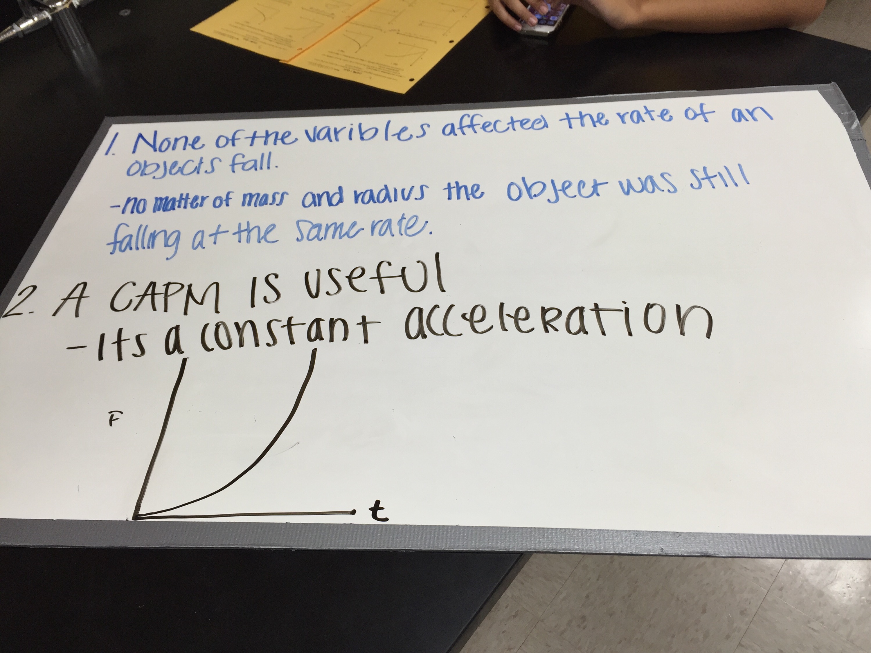
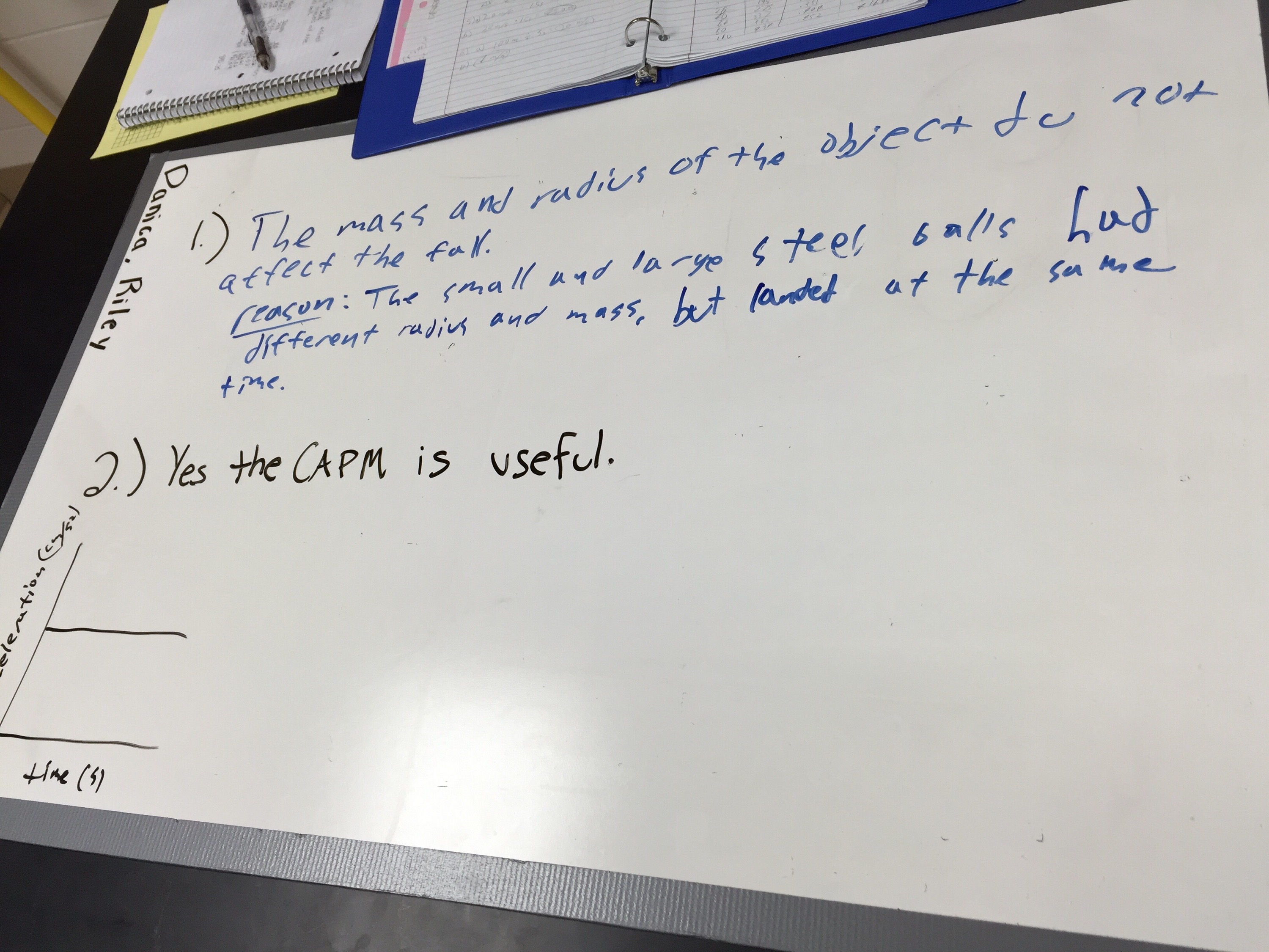
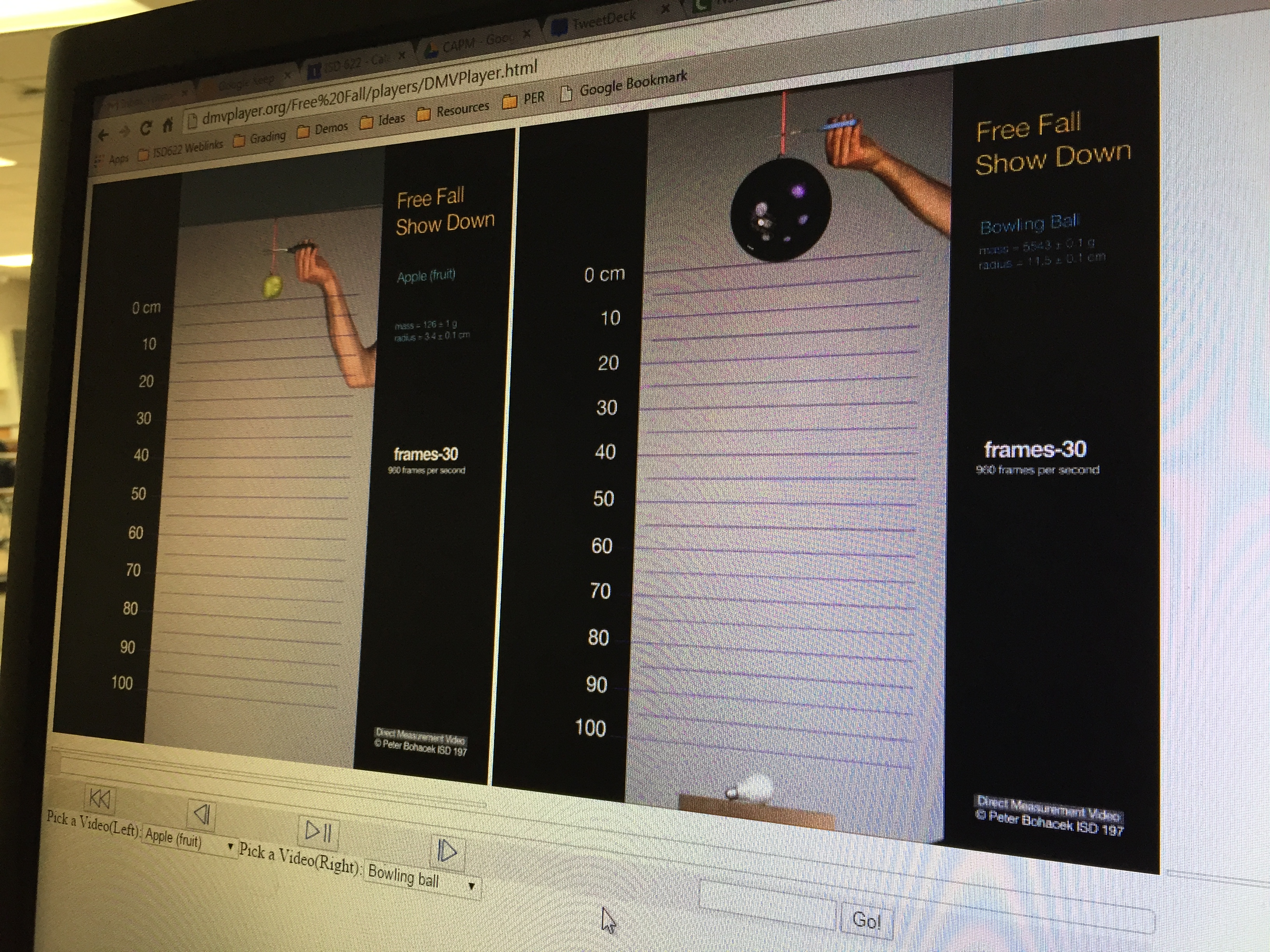
Physics: Acceleration Practical

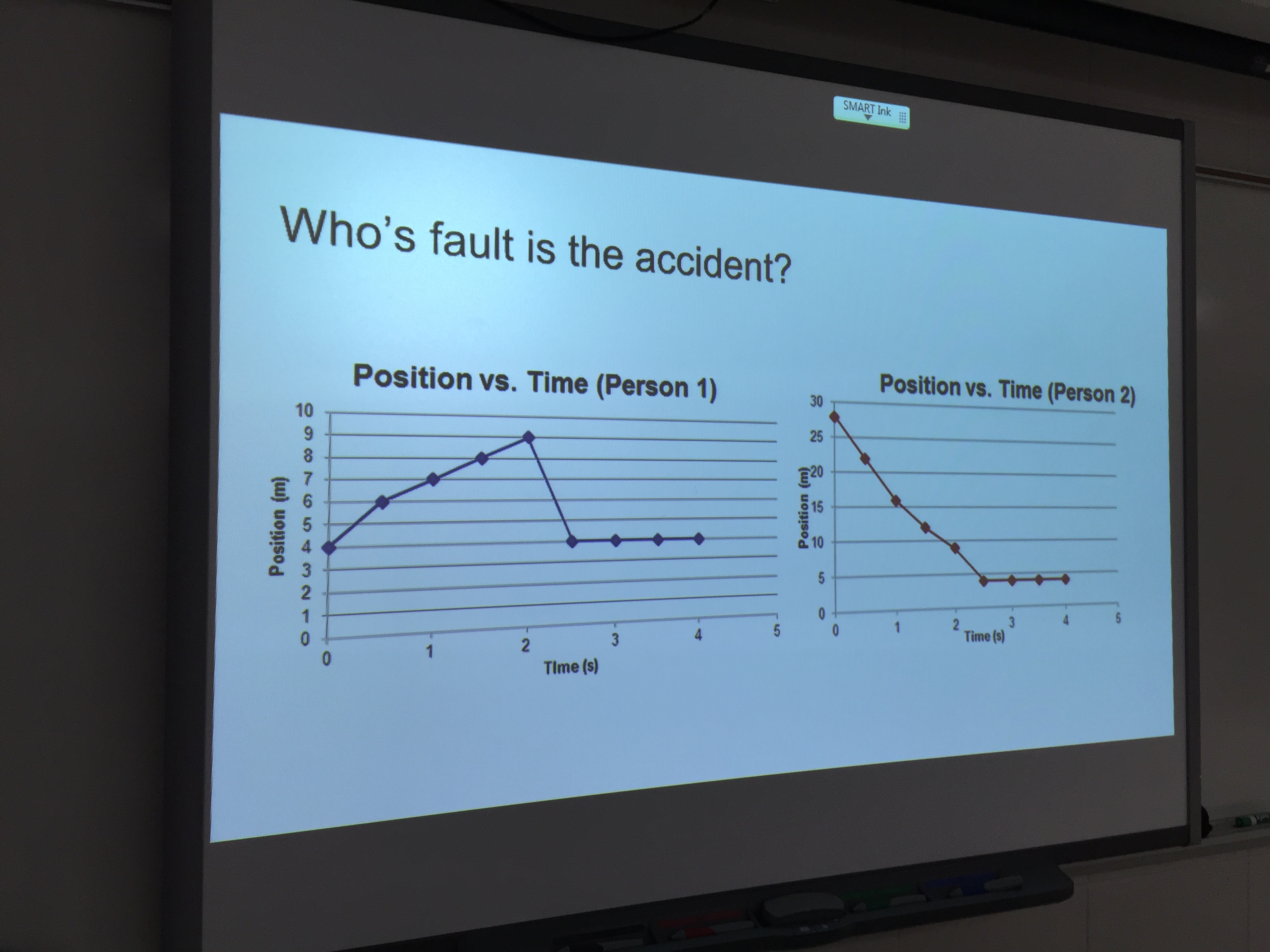
For most of the hour, students started working on a lab practical where they will roll a marble down a ramp so that it lands in a tumble buggy as it drives past. As a class, we collected the data students need to get the speed of the buggy and the acceleration of the marble, then students drew a random starting position for either the marble or buggy. I introduced the practical very clumsily in my first class, so I’ll need to do some clean up and clarification when we get back to the practical on Friday.

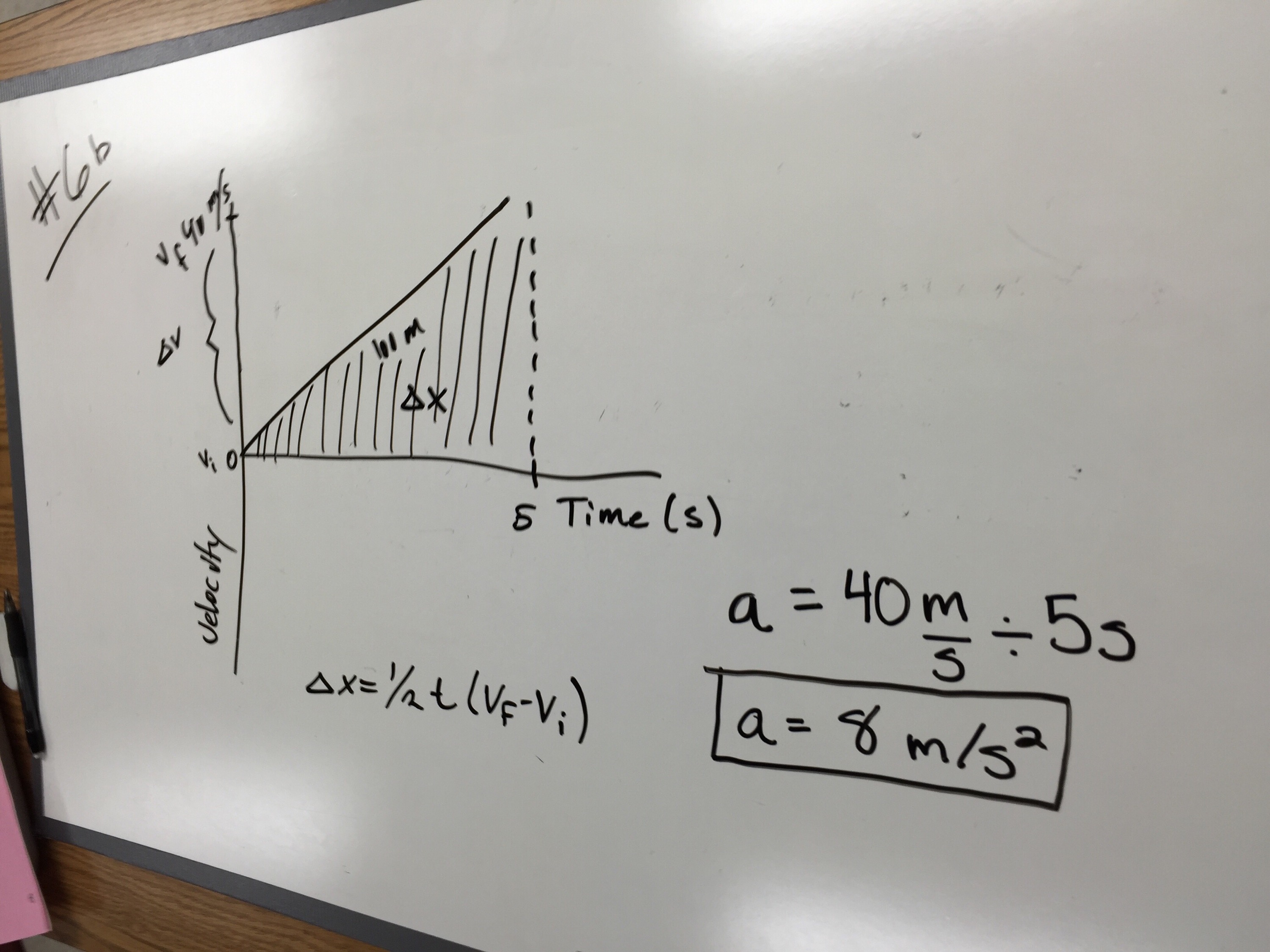
The first part of the lesson was finishing yesterday’s whiteboard presentations and produced one of my favorite moments of the day. When preparing their whiteboard yesterday, one group made the very common mistake of using v = d/t to find the final velocity of an accelerating object. In their quick conversation, they realized their answer didn’t make sense with the other values and were able to correct it. That group was brave enough to share that mistake, as well as how they caught it, when they presented the problem.

Day 16: Engineering Design Challenge & Communicating Solutions

Physical Science: Engineering Design Challenge

We teach forces using a project-based unit centered on an engineering desig challenge. Today, I introduced the challenge: students must make a cargo carrier that attaches to a truck will keep an egg intact in a head on collision. We spent some time today brainstorming what the customer may be interested in and what kind of background knowledge will be necessary for the task.


Physics: Comminicating Solutions

We spent some time on the importance of communication in science and connected that to what it means to show your work clearly in physics. From there, students whiteboarded the problems they worked on yesterday with clear communication in mind. This lead students to bemoan the lack of color choices in my marker bin.

Day 15: Interpreting Motion Graphs & Graphical Solutions

Physical Science: Interpreting Motion Graphs

To wrap-up the unit on motion, I used an activity from the 2014 EngrTEAMS summer institute at the University of Minnesota. Given position vs. time graphs for two cyclists, I first had them identify when they collided. Next, students had to decide who was at fault and construct an argument based on the graphs. There was a wide range of answers that used a lot of different evidence from the graphs, which is exactly what I was hoping for.

argumentation

Physics: Graphical Solutions

Now that students have a pretty good handle on velocity vs. time graphs, they took their first stab at solving problems using graphical solutions. By the end of the hour, most students seemed pretty comfortable with this approach. I’m sure it helped that our AP Calculus teacher has students do quite a few kinematics problems and uses graphical solutions as a stepping stone to integrals. Its almost like physics and calculus are related!

graphical solution

Day 14: Free Fall & Graph Stacks

Physical Science: Free Fall

Today, students explored the variables that affect how quickly an object falls. Class began with a brainstorming session to come up with as many variables as possible that might affect how quickly an object falls. Each group then picked two variables and designed their own tests. Most groups focused on weight and surface area, but one group did some quick research on different paper airplane designs, then compared different wing shapes.

IMG_0237

Physics: Graph Stacks

Starting from position vs. time graphs, students worked on generating stacks of kinematic graphs (matching position vs. time, velocity vs. time, and acceleration vs. time graphs). Students also drew the motion maps and wrote verbal descriptions of the motion. My students who’ve taken calculus almost all started with the graphs, then had to think a bit on the motion maps and the verbal descriptions. My students currently in pre-calc tended to start with the motion maps and written descriptions, then use those to make the graphs. Both groups of students had some good conversations as they worked through the task.

Day 13: Graphing Challenge & Motion Maps

Physical Science: Graphing Challenge

To get a little more practice with position vs. time graphs before we move on to free fall, the class went to the library to play Matt Blackman’s Action Graphing. My strongest students whipped through the early levels and got some exposure to velocity vs. time graphs as well as some calculations on graphs that show acceleration, which I normally don’t go into in this course due to time. Some of my students who need a little more time to master things started out using a lot of guess and check in the game, but were able to calculate correctly and consistently by the end of the period.

IMG_0233

Physics: Acceleration Motion Maps

Today, students drew motion maps and sketched graphs for variations on a sphere rolling along a ramp, then we got out the motion detector to check a few of them. I’ve got a number students who took AP Calculus BC last year who were able to work through most of the graphs pretty easily, but some of them retain some important misconceptions. I made sure we spent a lot of time on a cart that rolled up the ramp, then back down, because several students were adamant that a negative acceleration must always mean the object is slowing down. Even for some of the students who talk about velocity and acceleration as derivatives, the graphs for the cart going up and back down were surprising.

Screen Shot 2015-09-24 at 12.15.14 PM

Day 12: Graph Matching & Board Meeting

My phone had a mishap with a drink this afternoon, so the photos I took are out of reach for now.

Physical Science: Graph Matching

Today I got out the motion detector to have students do some graph matching. My department doesn’t have enough LabQuests to do one per group, so the lesson was a mix between students in groups and testing predictions with the motion detector as a whole class. We hadn’t gone into the significance of the sign of the slope on a position time graph, so I had students start by sketching predicted position vs. time graphs for several written descriptions, with objects traveling both towards and away from the motion detector before having students walk the graphs from the Vernier activity.  Students loved the motion detector and I had no shortage of volunteers to try and walk the graphs.

Physics: Board Meeting

Students prepared whiteboards with their position vs. time graphs and linearized graphs from rolling carts down ramps. I’d hoped to include velocity vs. time graphs, as well, but the computer issues yesterday meant students just didn’t have time to produce those graphs. For the discussion, I used Casey Rutherford’s observations, claims, and evidence framework. I also took time at several points in the discussion to have students discuss with their neighbors before sharing with the whole class. Compared to the first board meeting, students did a lot more talking and I did a lot less. When I did talk, I asked much broader questions than last time. I’m pleased with the improvements both my students and I have made since the first board meeting.

Day 11: More Motion Graphs & Data Analysis

Physical Science: Interpreting Motion Graphs

Students worked through a few questions based on a graph of an imaginary bike race. After a few straightforward interpretation questions like who started out the fastest and who finished first, I borrowed a page from Frank Noschese and asked students to come up with a few different ways to find the average velocity of Barry. Students then tested their approaches by using each speed to predict how long it should take Barry to finish the race. The average speed found by taking the total distance over the total time gave a result closest to his actual time, so students decided that is what we should use for average speed. They also liked that this was the easiest of all the approaches 🙂

The Bike Race

Physics: Data Analysis

Students graphed the position vs. time data they collected yesterday for a cart rolling down a ramp. I always waffle over whether to reserve a computer lab or a netbook cart for things like this. Our netbooks are a few years old and not terribly reliable, so using them means some technical glitches and frustration that can usually be avoided in a computer lab. On the other hand, I knew that some groups would need to collect additional data or to re-measure a few points. I could have clued those groups in yesterday, but I’d much rather they use their graph to see a need for additional data and make the choice themselves, which means they need access to lab equipment while graphing. Regardless of the netbook issues, just about every group got a position vs. time graph and (hopefully) knows what they need to do to make a linearized graph. Tomorrow, we’ll prep whiteboards and discuss the results.