Physical Science: Motion Maps

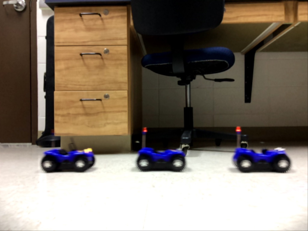
Students began by finding the slopes of the lines they graphed on Friday. I’d previously had them find the average speed of each walker, so it was a pretty easy leap to slope means velocity. Next, I had students observe some constant speed buggies and an accelerating, then showed them images I’d made with Motion Shot. That lead nicely into an activity where students produced position vs. time graphs from a motion map to compare an object with a constant speed to one with a changing speed. I’ve done the activity for several years, but this is the first time I felt like students really “got” what the motion map was showing; I think the Motion Shot photos I used were a big factor in that shift.

Physics: Building the Constant Acceleration Model

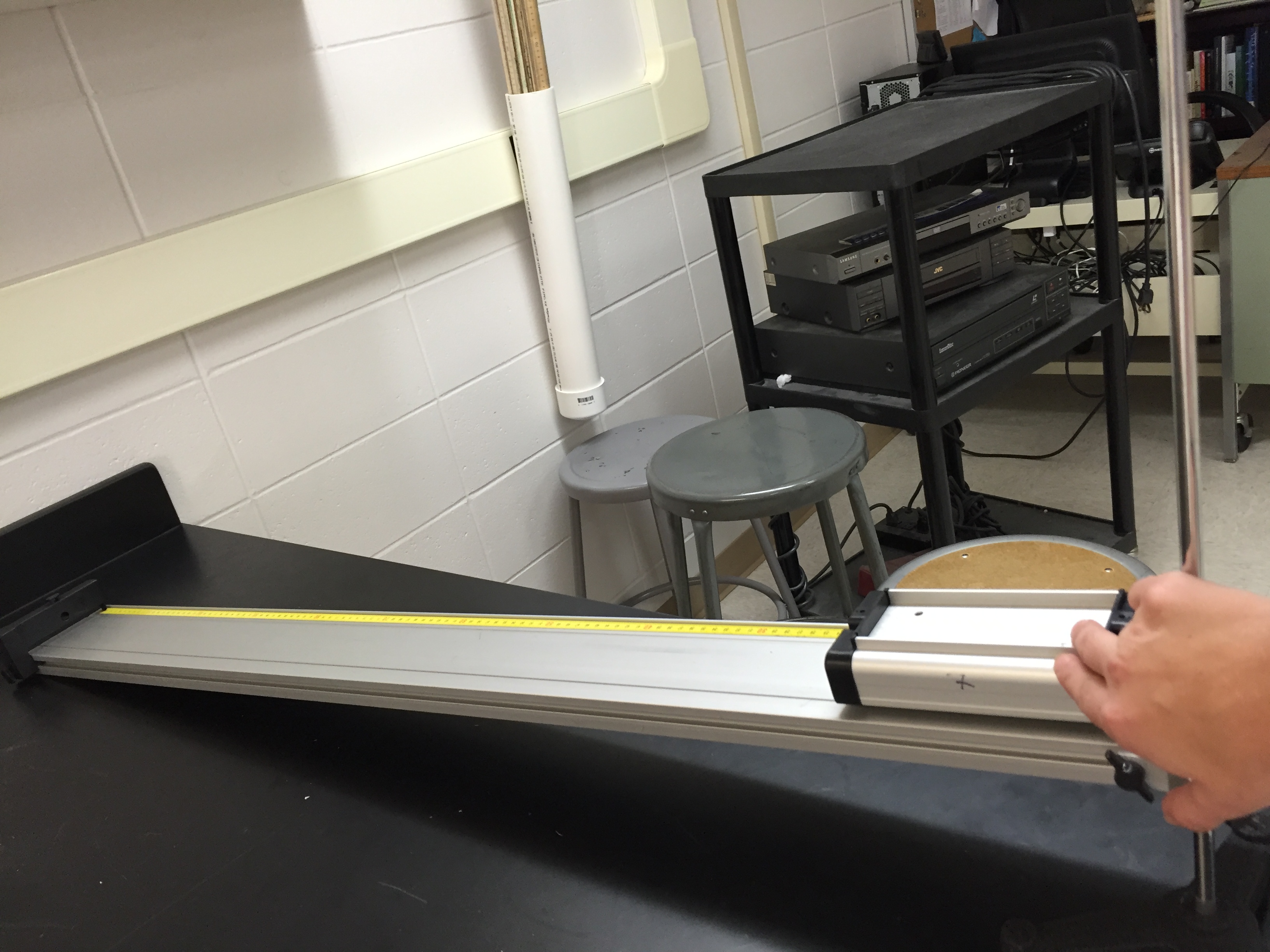
Today, students began building the constant acceleration model. We started by reviewing the limitations of the constant velocity model, then I turned them loose to collect data that would allow them to model the motion of a cart down the ramp. My students were great about diving in to play with the equipment in order to come up with a good approach.